Linear Regression in R for Gentle Souls

In statistics, linear regression is a linear approach for modelling the relationship between a response and one or more explanatory variables. It is fairly intuitive and works fairly well in the cases where a linear relationship exists between variables.

Linear regression is a statistical technique used to model the relationship between a dependent variable (also known as the response variable) and one or more independent variables (also known as predictor variables). The goal of linear regression is to find the best linear relationship between the dependent variable and the independent variables.

In simple linear regression, there is only one independent variable. The relationship between the dependent variable and the independent variable can be represented by a straight line, hence the term “linear” regression. The equation for a simple linear regression model is:

Y = a + bX + e

Where:

Y is the dependent variable
X is the independent variable
a is the intercept (the value of Y when X=0)
b is the slope (the change in Y for a one-unit change in X)
e is the error term (the difference between the predicted value of Y and the actual value of Y)

In multiple linear regression, there are multiple independent variables. The equation for a multiple linear regression model is similar to the simple linear regression model, but with multiple independent variables:

Y = a + b1X1 + b2X2 + … + bnXn + e

Where:

Y is the dependent variable
X1, X2, …, Xn are the independent variables
a is the intercept
b1, b2, …, bn are the slopes
e is the error term

To build a linear regression model in R, you can use the lm() function. Here’s an example:

# Load necessary libraries
install.packages('ggplot2')

Installing package into '/cloud/lib/x86_64-pc-linux-gnu-library/4.4'
(as 'lib' is unspecified)

library(ggplot2)

# Load the iris dataset
data(iris)

# Fit a simple linear regression model
model <- lm(Petal.Width ~ Petal.Length, data = iris)

# Show the model summary
summary(model)


Call:
lm(formula = Petal.Width ~ Petal.Length, data = iris)

Residuals:
     Min       1Q   Median       3Q      Max 
-0.56515 -0.12358 -0.01898  0.13288  0.64272 

Coefficients:
              Estimate Std. Error t value Pr(>|t|)    
(Intercept)  -0.363076   0.039762  -9.131  4.7e-16 ***
Petal.Length  0.415755   0.009582  43.387  < 2e-16 ***
---
Signif. codes:  0 '***' 0.001 '**' 0.01 '*' 0.05 '.' 0.1 ' ' 1

Residual standard error: 0.2065 on 148 degrees of freedom
Multiple R-squared:  0.9271,    Adjusted R-squared:  0.9266 
F-statistic:  1882 on 1 and 148 DF,  p-value: < 2.2e-16

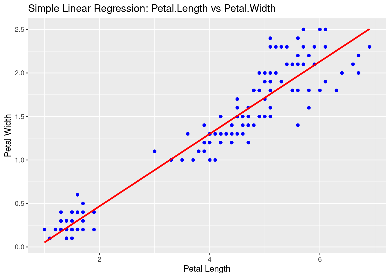
# Plot with regression line
ggplot(iris, aes(x = Petal.Length, y = Petal.Width)) +
  geom_point(color = "blue") +
  geom_smooth(method = "lm", se = FALSE, color = "red") +
  labs(title = "Simple Linear Regression: Petal.Length vs Petal.Width",
       x = "Petal Length",
       y = "Petal Width")

`geom_smooth()` using formula = 'y ~ x'

We first load the data and build a simple linear regression model using the lm() function. We then view the summary of the model to see the coefficients, R-squared value, and other statistics. We can then make predictions using the model by creating a new data frame with the independent variable values we want to predict for, and using the predict() function to generate the predicted values.

Final Thought

Be advised that a linear relationship does not always exist between two variables, yet they are related. Linear regression is just one tool of many that can be utilized to describe the reality of your data.